5.1.1 手法1(部分空間法)

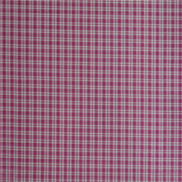
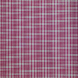
【テクスチャ構造の低減処理】

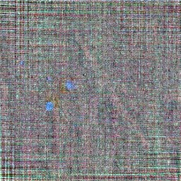
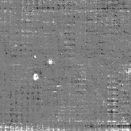
2種類の対象画像(縦256$\times$横256画素)それぞれに対し，2.2節で述べた手法を用いてテクスチャ構造の低減処理を行った．まず，図6に示す縦方向および横方向の1次元パワースペクトルのピークよりテクスチャ構造の周期を求める．2種類の対象画像それぞれをテクスチャ構造の2周期分に相当する縦22$\times$横21画素のブロックに分割し，式(7)$\sim$(9)を用いて固有値$\lambda_i$と固有ベクトル $u$$_i$を求めた．求めた固有値を降順にソートし，大きい固有値に対応する固有ベクトル画像を図7(a)$\sim$(e)に，小さい固有値に対応する固有ベクトル画像を図7(f)$\sim$(j)に示す．図7より，大きい固有値に対応する固有ベクトル画像が対象画像の平均的なテクスチャ構造を表していることがわかる．また，固有値を降順にソートした値の変化を図8に，累積寄与率の値の変化を図9に示す．図8より，9番目の固有値で大きく減少していることと，図9より，累積寄与率が10番目以降漸近的に増加していることから，式(10)の部分空間次元数$P$を10として以下の処理を行った．白色LEDを光源として撮影した布画像の近似画像を図10(a)に，テクスチャ低減画像を図11(a)に示す．同様に，近紫外LEDを光源として撮影した布画像の近似画像を図10(b)に，テクスチャ低減画像を図11(b)に示す．図11より，対象画像のテクスチャ成分が低減されていることが確認できる．

図 6: パワースペクトル

(a)縦方向	(b)横方向

図 7: 固有ベクトル画像

(a) $u$$_0$	(b) $u$$_1$	(c) $u$$_2$	(d) $u$$_3$	(e) $u$$_4$

(f) $u$$_{50}$	(g) $u$$_{51}$	(h) $u$$_{52}$	(i) $u$$_{53}$	(j) $u$$_{54}$

図 8: 固有値

図 9: 累積寄与率

図 10: 近似画像

(a)白色LED	(b)近紫外LED

図 11: テクスチャ低減画像

(a)白色LED	(b)近紫外LED

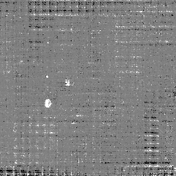
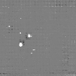
【PCAを用いた無相関化】

2種類のテクスチャ低減画像それぞれのRGB成分同士の差分の三乗の画素値ベクトル $y$$[m,n]$に対し，3節で述べた手法を用いて無相関化を行った結果を図12に示す．図12より，汚れ部分が全ての成分で鮮明化されていることが確認できる．

図 12: 無相関化成分画像

(a)第0成分	(b)第1成分	(c)第2成分

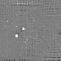
【ICAを用いた独立成分の抽出】

無相関化を行ったベクトル $Y$$[m,n]$に対し，4節で述べた手法を用いて独立な成分に分解した結果を図13に示す．第0成分で汚れ部分が鮮明化されていることが確認できる．

図 13: 独立成分画像

(a)第0成分	(b)第1成分	(c)第2成分